% Use of CVX to maximize G/Q for a rectangle dipole geometry
% see Sec. VII.B in
% M. Gustafsson, D. Tayli, C. Ehrenborg, M. Cismasu, S. Nordebo
% Tutorial on antenna current optimization using MATLAB and CVX
% 2015

clear all
k1=0.05*2*pi; k2=0.5*2*pi; kN=50; lx=1; ly=0.5; Nx=32; Ny=16; % 0.5 rectangle
% k1=0.05*2*pi; k2=0.5*2*pi; kN=50; lx=1; ly=0.5; Nx=64; Ny=32; % 0.5 rectangle
lib = '..\data';  % path to the data library
% Calc_RX_matrices_rec(k1,k2,kN,lx,ly,Nx,Ny,lib);
% comment out after evaluation of the R,Xe,Xm matrices

farfieldtype = 'farfield';
farfieldtype = 'sphmode';

solvertype = 1; % CVX with quad_form
solvertype = 2; % CVX with norm
solvertype = 3; % Newton iteration
solvertype = 3;

a = 0.5;  % initiation for the Newton iterations
kres = zeros(1,kN); %  matrix with wavenumbers
GoQres = zeros(1,kN); % matrix with G/Q
Qres = zeros(1,kN); % matrix resulting Q
Dres = zeros(1,kN); % matrix with resulting D
for kn=1:kN
    % load the data files
    load(strcat(lib,'/RowRX_rec_x=1_y=0p5_Nx=32_Ny=16_k=0p31416_3p1416_50_',num2str(kn)));
%     load(strcat(lib,'/RowRX_rec_x=1_y=0p5_Nx=64_Ny=32_k=0p31416_3p1416_50_',num2str(kn)));
    % constructs the reactance matrices Xe, Xm from the computed data
    [Xe,p] = RX_rec_sym2full(Xe11,Xe12,Xe22,bas.BxNN,bas.ByNN,meshp.txN,meshp.tyN,2);
    [Xm,p] = RX_rec_sym2full(Xm11,Xm12,Xm22,bas.BxNN,bas.ByNN,meshp.txN,meshp.tyN,2);
    [Rr,p] = RX_rec_sym2full(Rr11,Rr12,Rr22,bas.BxNN,bas.ByNN,meshp.txN,meshp.tyN,0);
    switch farfieldtype(1)
        case 'f'
            % computed the far-field matrix for
            evh = [1 0 0];
            rvh = [0 0 1];
            [F] = farfieldmatrix(kl,bas,meshp,evh,rvh);
        case 's'
            % computed the far-field matrix for spherical mode
            sphn = 6; % x-directed electric dipole
            F = sphmodematrix(kl,bas,meshp,sphn);
    end

    switch solvertype
        case 1
            % CVX code for maximization of G/Q
            cvx_begin
               variable I(N) complex;     % current
               variable w;                % n. stored energy
               minimize w
               subject to
                 quad_form(I,Xe) <= w;    % n. stored E energy
                 quad_form(I,Xm) <= w;    % n. stored M energy
                 F*I == -1i;              % far-field
            cvx_end
            GoQ = 4*pi/(w*eta0)           % bound on G/Q
        case 2
            % CVX code for maximization of G/Q
            sqrtXe = sqrtm(Xe);
            sqrtXm = sqrtm(Xm);
            cvx_begin
               variable I(N) complex;  % current
               variable w;             % sqrt stored energy
               minimize w
               subject to
                 norm(sqrtXe*I) <= w;  % sqrt stored E energy
                 norm(sqrtXm*I) <= w;  % sqrt stored M energy
                 F*I == -1i;           % far-field
            cvx_end
            w = w*w;                   % n. stored energy
            GoQ = 4*pi/(w*eta0)        % bound on G/Q
        case 3
            gap0 = 1e-7;        % max gap in G/Q
            adiff0 = 1e-7;      % max difference in a
            m0 = 20;            % max number of Newton it
            abound1 = 0.01;     % boundary for the Newton it
            [a,GoQai,m,GoQrgap,adiff] = AntennaGoQ_NewtonIt(a,Xe,Xm,F,gap0,adiff0,m0,abound1);
            Xa = a*Xe+(1-a)*Xm;
            J = Xa\F';
            d = 1/real(F*J);                % dual value
            I = -1i*d*J;                  % current
            P = abs(F*I)^2*4*pi/eta0;% n. rad. int.
            QoGe = real(I'*Xe*I)/P;          % Qe/G
            QoGm = real(I'*Xm*I)/P;          % Qm/G
            GoQaa = 1/max(QoGe,QoGm);        % G/Q
            GoQdd = 1/(a*QoGe+(1-a)*QoGm);   % dual G/Q
            GoQ = GoQaa;
            Prad = real(I'*Rr*I);
            D = 4*pi/Prad/eta0;          % directivity
            Qe = real(I'*Xe*I)/Prad;          % Qe/G
            Qm = real(I'*Xm*I)/Prad;          % Qe/G
            Q = max(Qe,Qm);
    end

    % antenna parameters from the max. G/Q problem
    P = abs(F*I)*abs(F*I)/2/eta0; % radiation intensity
    Pr = real(I'*Rr*I)/2;         % radiated power
    D = 4*pi*P/Pr;                 % res. directivity
    We = real(I'*Xe*I)/4/kl;      % stored E energy
    Wm = real(I'*Xm*I)/4/kl;      % stored M energy
    W = max(We,Wm);               % stored energy
    Q = 2*kl*W/Pr;                 % Q
    Qe = 2*kl*We/Pr;              % Q electric
    Qm = 2*kl*Wm/Pr;              % Q magnetic
    kres(kn) = kl;
    GoQres(kn) = GoQ;
    Qres(kn) = Q;
    Dres(kn) = D;
    disp(strcat('kn/kN=',num2str(kn/kN,'%0.2f')))
end
% evaluates the D/Q from the forward scattering bound
[DoQFS,QFS,ka,polarizability] = AntennaQ(lx, ly, 'rectangle_v', 3e8*kres/2/pi);

% plots G/Q from antenna current optimization and G/Q from forward scattering
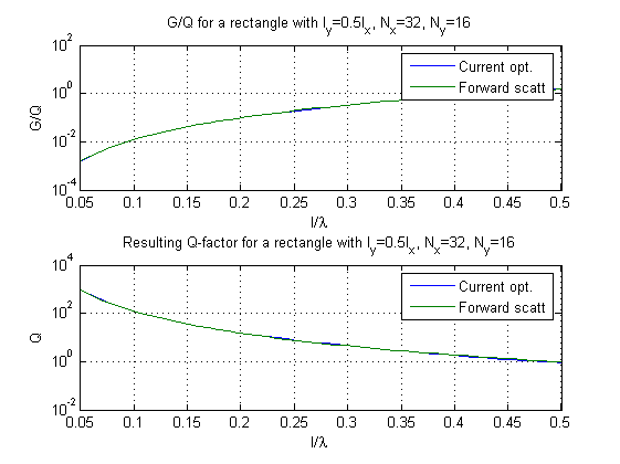
figure(1); clf
subplot(2,1,1)
semilogy(kres/2/pi,GoQres,kres/2/pi,DoQFS)
grid on
xlabel('l/\lambda')
ylabel('G/Q')
legend('Current opt.','Forward scatt')
title(strcat('G/Q for a rectangle with l_y=',num2str(ly),'l_x, N_x=',num2str(Nx),', N_y=',num2str(Ny)))

subplot(2,1,2)
semilogy(kres/2/pi,Qres,kres/2/pi,QFS)
grid on
xlabel('l/\lambda')
ylabel('Q')
legend('Current opt.','Forward scatt')
title(strcat('Resulting Q-factor for a rectangle with l_y=',num2str(ly),'l_x, N_x=',num2str(Nx),', N_y=',num2str(Ny)))

% plots G/Q from antenna current optimization and forward scattering
% normalized with the electrical size k^3a^3
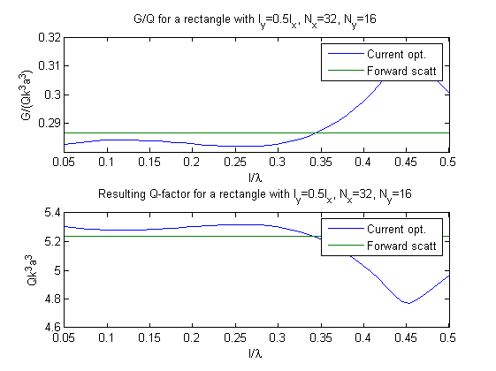
figure(2); clf
rad = sqrt(lx^2+ly^2)/2;  % radius of the circumcribing sphere
ka3 = kres.^3*rad^3;
subplot(2,1,1)
plot(kres/2/pi,GoQres./ka3,kres/2/pi,DoQFS./ka3)
legend('Current opt.','Forward scatt')
title(strcat('G/Q for a rectangle with l_y=',num2str(ly),'l_x, N_x=',num2str(Nx),', N_y=',num2str(Ny)))
xlabel('l/\lambda')
ylabel('G/(Qk^3a^3)')
subplot(2,1,2)
plot(kres/2/pi,Qres.*ka3,kres/2/pi,QFS.*ka3)
legend('Current opt.','Forward scatt')
title(strcat('Resulting Q-factor for a rectangle with l_y=',num2str(ly),'l_x, N_x=',num2str(Nx),', N_y=',num2str(Ny)))
xlabel('l/\lambda')
ylabel('Qk^3a^3')

kn/kN=0.02
kn/kN=0.04
kn/kN=0.06
kn/kN=0.08
kn/kN=0.10
kn/kN=0.12
kn/kN=0.14
kn/kN=0.16
kn/kN=0.18
kn/kN=0.20
kn/kN=0.22
kn/kN=0.24
kn/kN=0.26
kn/kN=0.28
kn/kN=0.30
kn/kN=0.32
kn/kN=0.34
kn/kN=0.36
kn/kN=0.38
kn/kN=0.40
kn/kN=0.42
kn/kN=0.44
kn/kN=0.46
kn/kN=0.48
kn/kN=0.50
kn/kN=0.52
kn/kN=0.54
kn/kN=0.56
kn/kN=0.58
kn/kN=0.60
kn/kN=0.62
kn/kN=0.64
kn/kN=0.66
kn/kN=0.68
kn/kN=0.70
kn/kN=0.72
kn/kN=0.74
kn/kN=0.76
kn/kN=0.78
kn/kN=0.80
kn/kN=0.82
kn/kN=0.84
kn/kN=0.86
kn/kN=0.88
kn/kN=0.90
kn/kN=0.92
kn/kN=0.94
kn/kN=0.96
kn/kN=0.98
kn/kN=1.00

Published with MATLAB® R2013b