maxGoQ_CVX_1

% Use CVX to maximize G/Q for a strip dipole geometry
% see Sec. VII.B in
% M. Gustafsson, D. Tayli, C. Ehrenborg, M. Cismasu, S. Nordebo
% Tutorial on antenna current optimization using MATLAB and CVX
% 2015

clear all
k1=0.5*2*pi; k2=k1; kN=1; lx=1; ly=0.02; Nx=100; Ny=1; % half-a-wavelenth strip dipole
lib = '..\data';  % path to the data library
Calc_RX_matrices_rec(k1,k2,kN,lx,ly,Nx,Ny,lib);
% load the data files
load(strcat(lib,'/RowRX_rec_x=1_y=0p02_Nx=100_Ny=1_k=3p1416'));
% constructs the reactance matrices Xe, Xm from the computed data
[Xe,p] = RX_rec_sym2full(Xe11,Xe12,Xe22,bas.BxNN,bas.ByNN,meshp.txN,meshp.tyN,2);
[Xm,p] = RX_rec_sym2full(Xm11,Xm12,Xm22,bas.BxNN,bas.ByNN,meshp.txN,meshp.tyN,2);
[Rr,p] = RX_rec_sym2full(Rr11,Rr12,Rr22,bas.BxNN,bas.ByNN,meshp.txN,meshp.tyN,2);
if 1
    % compute the far-field matrix for
    evh = [1 0 0];
    rvh = [0 0 1];
    F = farfieldmatrix(kl,bas,meshp,evh,rvh);
else
    % compute the far-field matrix for spherical mode
    sphn = 6; % x-directed electric dipole
    F = sphmodematrix(kl,bas,meshp,sphn);
end

% CVX code for maximization of G/Q
cvx_begin
   variable I(N) complex;     % current
   variable w;                % n. stored energy
   minimize w
   subject to
     quad_form(I,Xe) <= w;    % n. stored E energy
     quad_form(I,Xm) <= w;    % n. stored M energy
     F*I == -1i;              % far-field
cvx_end
GoQ = 4*pi/(w*eta0)           % bound on G/Q

% plot the current density
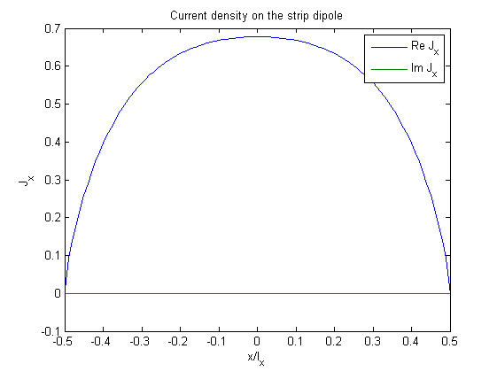
figure(1); clf
x = linspace(-lx/2,lx/2,N+2);       % x coordinates
plot(x,real([0; I/dy; 0]),x,imag([0; I/dy; 0]))
title('Current density on the strip dipole')
xlabel('x/l_x')
ylabel('J_x')
legend('Re J_x','Im J_x')

% antenna parameters from the max. G/Q problem
P = abs(F*I)*abs(F*I)/2/eta0; % radiation intensity
Pr = real(I'*Rr*I)/2;         % radiated power
D = 4*pi*P/Pr                 % res. directivity
We = real(I'*Xe*I)/4/kl;      % stored E energy
Wm = real(I'*Xm*I)/4/kl;      % stored M energy
W = max(We,Wm);               % stored energy
Q = 2*kl*W/Pr                 % Q
Qe = 2*kl*We/Pr;              % Q electric
Qm = 2*kl*Wm/Pr;              % Q magnetic

Nx =
   100
Ny =
     1
kn/kN=1.000, t=0:0:1, rt=0:0:0
 
Calling SDPT3 4.0: 405 variables, 202 equality constraints
   For improved efficiency, SDPT3 is solving the dual problem.
------------------------------------------------------------

 num. of constraints = 202
 dim. of socp   var  = 400,   num. of socp blk  =  2
 dim. of linear var  =  2
 dim. of free   var  =  3 *** convert ublk to lblk
*******************************************************************
   SDPT3: Infeasible path-following algorithms
*******************************************************************
 version  predcorr  gam  expon  scale_data
    NT      1      0.000   1        0    
it pstep dstep pinfeas dinfeas  gap      prim-obj      dual-obj    cputime
-------------------------------------------------------------------
 0|0.000|0.000|8.3e+03|8.5e+02|4.4e+04| 4.032922e+01  0.000000e+00| 0:0:00| chol  1  1 
 1|0.972|0.965|2.4e+02|2.9e+01|2.9e+03| 2.425279e+01 -1.675440e+03| 0:0:00| chol  1  1 
 2|1.000|0.350|8.2e-06|1.9e+01|1.2e+03| 6.053100e+00 -1.136137e+03| 0:0:00| chol  1  1 
 3|1.000|0.944|7.1e-06|1.1e+00|7.0e+01| 1.621333e+00 -6.327848e+01| 0:0:00| chol  1  1 
 4|0.980|0.933|5.4e-07|7.2e-02|4.7e+00| 1.124395e+00 -3.219186e+00| 0:0:00| chol  1  1 
 5|0.988|0.983|1.8e-07|1.2e-03|7.9e-02| 1.112303e+00  1.040646e+00| 0:0:00| chol  1  1 
 6|0.954|0.049|1.5e-06|1.2e-03|7.6e-02| 1.111034e+00  1.044105e+00| 0:0:00| chol  1  1 
 7|1.000|0.453|4.6e-08|6.4e-04|4.2e-02| 1.110706e+00  1.074286e+00| 0:0:00| chol  1  1 
 8|0.808|0.327|4.0e-08|4.3e-04|2.8e-02| 1.109769e+00  1.086000e+00| 0:0:00| chol  1  1 
 9|1.000|0.298|2.3e-08|3.0e-04|2.0e-02| 1.109392e+00  1.093013e+00| 0:0:00| chol  1  1 
10|0.996|0.650|3.6e-09|1.1e-04|7.0e-03| 1.108967e+00  1.103484e+00| 0:0:00| chol  1  1 
11|0.635|0.489|4.6e-09|5.4e-05|3.6e-03| 1.108771e+00  1.106069e+00| 0:0:00| chol  1  1 
12|0.461|0.678|5.6e-09|1.8e-05|1.2e-03| 1.108687e+00  1.107807e+00| 0:0:00| chol  1  1 
13|0.577|0.742|3.1e-09|4.6e-06|3.2e-04| 1.108649e+00  1.108417e+00| 0:0:00| chol  1  1 
14|0.876|0.800|7.2e-10|9.4e-07|6.4e-05| 1.108637e+00  1.108591e+00| 0:0:00| chol  1  1 
15|0.985|0.949|1.1e-10|7.1e-08|3.4e-06| 1.108636e+00  1.108634e+00| 0:0:00| chol  1  1 
16|0.995|0.963|9.5e-12|3.3e-09|1.4e-07| 1.108636e+00  1.108636e+00| 0:0:00| chol  1  1 
17|1.000|0.933|3.9e-11|1.7e-10|1.0e-08| 1.108636e+00  1.108636e+00| 0:0:00|
  stop: max(relative gap, infeasibilities) < 1.49e-08
-------------------------------------------------------------------
 number of iterations   = 17
 primal objective value =  1.10863592e+00
 dual   objective value =  1.10863592e+00
 gap := trace(XZ)       = 1.01e-08
 relative gap           = 3.14e-09
 actual relative gap    = 1.80e-09
 rel. primal infeas     = 3.88e-11
 rel. dual   infeas     = 1.66e-10
 norm(X), norm(y), norm(Z) = 7.7e+02, 8.5e-01, 1.0e+00
 norm(A), norm(b), norm(C) = 3.0e+03, 3.6e+00, 3.5e+00
 Total CPU time (secs)  = 0.48  
 CPU time per iteration = 0.03  
 termination code       =  0
 DIMACS: 4.1e-11  0.0e+00  2.7e-10  0.0e+00  1.8e-09  3.1e-09
-------------------------------------------------------------------
------------------------------------------------------------
Status: Solved
Optimal value (cvx_optval): +0.0958593
 
GoQ =
    0.3480
D =
    1.6811
Q =
    4.8313